GNN-GRU pipeline for 3D trajectory forecasting
2025 · sole developer · PyTorch, PyTorch Geometric
Forecasting the 3D motion of many interacting articulated objects, where each object is a set of tracked points rather than a single centre of mass, and where the objects influence each other only when they are close.
Two-second comparison of real against predicted trajectories (video)
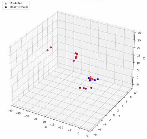
Blue circles are ground truth, red triangles are the prediction, dashed lines connect the same tracked point in both. The model is running open loop here: it has seen no ground truth since the first frame.
The problem
The input is a stream of frames. Each frame lists objects; each object is broken into parts, and each part carries a class, a stable identifier and a 3D position:
{"timestamp": 51, "objects": [
  {"instance_id": 3, "class_id": 1, "dot_id": 0, "pos": [12.4, 3.1, -8.7]},
  {"instance_id": 3, "class_id": 4, "dot_id": 2, "pos": [12.9, 3.4, -8.2]}
]}
Two properties make this harder than a standard sequence-forecasting task.
Objects interact, but only locally. Two objects fifty units apart do not affect each other. Modelling every pair is wasteful and, worse, teaches the network relationships that do not exist.
Objects are not points. Each one is a constellation of parts that move together but not rigidly. Predicting the centre of mass throws away exactly the information the task is about, and predicting every part independently throws away the fact that they belong to the same body.
Representation: two levels
The design separates where interaction happens from where dynamics happen.
Interaction is computed between objects. Each object collapses to a single anchor
position. The anchor is the mean of its parts with class_id == 1, falling back to the mean
of all valid parts when an object has no part of that class:
has_anchor = anchor_part_mask.any(dim=1, keepdim=True)
mask_for_mean = torch.where(has_anchor, anchor_part_mask, valid_part_mask)
mean_pos = (all_pos * mask_for_mean).sum(dim=1) / mask_for_mean.sum(dim=1).clamp(min=1)
The clamp(min=1) is there because an object can be entirely padding in a given frame, and
dividing by zero silently produces NaNs that only surface several epochs into training.
Dynamics are computed per part. Each object node carries all of its parts as features. A part is seven numbers: current position, previous-step velocity, and class:
features_tensor[:num_valid_parts] = torch.cat([pos_curr_t, prev_vel_t, class_ids_t], dim=1)
target_tensor[:num_valid_parts] = target_vel_t
mask_tensor[:num_valid_parts] = 1.0
Parts are padded to a fixed 200 per object with a mask, so a batch can hold objects of very different complexity.
Only parts that exist in three consecutive frames
Velocity needs the previous frame; the training target needs the next one. A part visible at
t but missing at t-1 has no velocity, and one missing at t+1 has no target. So each
training sample is built from the intersection of three frames:
valid_part_keys = sorted(list(
    parts_prev_indexed.keys() & parts_curr_indexed.keys() & parts_next_indexed.keys()
))
Parts are keyed by (class_id, dot_id) rather than by class alone, because an object can
have several parts of the same class and they must not be confused with one another.
The graph
Edges come from proximity, recomputed rather than fixed:
edge_index = radius_graph(anchor_positions, r=15.0, loop=False, max_num_neighbors=128)
Radius 15 with a neighbour cap of 128. The cap matters in dense frames: without it the attention layer occasionally received nodes with several hundred neighbours and memory use became unpredictable.
Model
per part:    Linear(7 → 64) → LeakyReLU → Linear(64 → 32)
per object:  flatten 200 × 32 → 6400
             GATv2Conv(6400 → 64, heads=4, concat=False, dropout=0.1)
             GRUCell(64, 64)                     ← carries state across timesteps
             Linear(64 → 128) → LeakyReLU → Linear(128 → 600) → reshape 200 × 3
Three deliberate choices.
The output is velocity, not position. Predicting absolute coordinates makes the network spend its capacity learning where the scene happens to be. Predicting displacement makes it learn how things move, which is the transferable part.
Attention over neighbours, not a fixed kernel. GATv2Conv lets an object weight its
neighbours differently. A nearby object on a collision course and a nearby object drifting
away are not equally relevant, and attention can express that where a mean or sum cannot.
Recurrence at the object level. The GRUCell carries a hidden state per object across
timesteps, so momentum and intent survive between frames instead of being re-derived from
two positions every step.
The hard part: the graph is a function of the prediction
During rollout the model is not just predicting coordinates. It predicts positions, and those positions determine which objects are neighbours in the next step:
new_pos_parts = current_positions + pred_vel
current_graph.x = torch.cat([new_pos_parts, pred_vel, class_ids_parts], dim=2)
new_anchor_pos = calculate_anchor_positions(current_graph.x, current_graph.mask)
current_graph.edge_index = radius_graph(new_anchor_pos, r=RADIUS, ...)
So error does not merely accumulate in the coordinates. It changes the topology. A small positional drift can push a pair of objects across the radius threshold, an edge appears or vanishes that should not have, and from then on the model is reasoning about a scene that never existed. This is the failure mode that makes long rollouts collapse, and it is not visible in single-step validation loss at all.
Training addresses it directly by unrolling during training rather than only at inference:
for k in range(TRAJECTORY_LENGTH):          # 10 steps
    pred_vel, h_sim = model(sim_graph_data.x, edge_index_sim, h_sim)
    ...
    use_teacher = random.random() < TEACHER_FORCING_RATIO      # 0.5
    next_vel_parts = target_vel if use_teacher else pred_vel
Half the steps feed the model its own output, including the rebuilt graph. It therefore learns to recover from its own drift rather than only from clean input.
Trained on 10 steps, evaluated on 20. The inference rollout is twice the horizon seen in training, with no teacher forcing anywhere, which is a real test of whether the model learned dynamics or memorised a short continuation.
Training details
| Optimiser | AdamW, learning rate 1e-3, weight decay 1e-5 |
| Schedule | 10 epochs linear warmup, then cosine decay over the remaining 140 |
| Epochs | 150 |
| Batch | 32 trajectory starts, sampled in shuffled order |
| Loss | MSE on velocity, masked, normalised by the number of valid parts |
| Stability | gradient clipping at norm 1.0; non-finite losses skipped rather than propagated |
The loss is normalised by the mask sum rather than by tensor size:
loss_per_node = loss_fn(pred_vel * mask, target_vel * mask)
sum_of_mask = mask.sum()
if sum_of_mask > 0:
    trajectory_loss += loss_per_node.sum() / sum_of_mask
Without that division, objects with many parts dominate the gradient purely because they contribute more terms, and the model quietly stops caring about small objects.
Validation
Loss curves are a poor way to judge a rollout: a model can hold a respectable MSE while producing motion that is obviously wrong to a human. So every run ends by writing an animation that draws ground truth and prediction in the same 3D axes, with a dashed line joining each tracked point to its own prediction, so the error is visible as a length rather than inferred from a number.
The camera angle and axis limits are recomputed per frame from the union of both point clouds, which keeps the comparison honest when the scene drifts out of the original bounds.
Predictions are also written to JSON in the same schema as the input, so a rollout can be fed back into any downstream tool that consumed the original data.
What I would do differently
The flatten is wasteful. Packing 200 parts × 32 dimensions into a single 6400-vector per object means an object with 12 parts carries 6400 numbers of which most are zero, and the representation is order-sensitive when it should be permutation-invariant. A pooled representation, or a second attention layer over the parts within an object, would be both smaller and more correct.
The batch loop is Python. Trajectory starts are iterated one at a time inside the batch
rather than being batched into a single graph. torch_geometric can batch disjoint graphs
into one, and doing so would remove most of the per-step overhead.
No physical constraints. Nothing prevents the model from predicting that two objects occupy the same space, or that a part detaches from its body. Rigid-distance penalties between parts of the same object would be cheap to add and would likely improve long rollouts more than extra capacity.
Fixed radius. 15.0 was chosen by inspection. Making the interaction radius learned, or at least tuned against rollout quality rather than single-step loss, is the obvious next experiment.